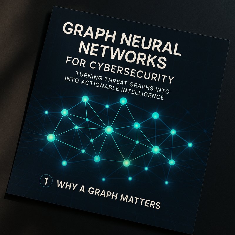
In the past decade, defenders have learned that security is not just about stopping a single attack; it’s about understanding how threats move, connect, and evolve. Traditional rule‑based systems can flag individual anomalies, but they often miss the bigger picture. That’s where Graph Neural Networks for Cybersecurity shine. By treating logs, network flows, and endpoint data as nodes and edges in a graph, GNNs can uncover hidden relationships and predict how an attacker might pivot.
Graph Neural Networks for Cybersecurity are already helping organizations reduce false positives, identify lateral movement, and map supply‑chain risk. In this guide we’ll break down how to build a threat‑graph pipeline, dive into real‑world examples, and show you how to start using GNNs without a PhD.
1️⃣ Why a Graph Matters
A graph is a natural way to model the cybersecurity universe. Think of each device, process, or user as a node, and every interaction—like an API call, a DNS query, or a file access—as an edge. When you layer this structure with attributes (time stamps, severity scores, etc.), you get a rich, interconnected view of your environment.
Graph Neural Networks for Cybersecurity learn from this structure. Unlike flat machine‑learning models that treat each event in isolation, GNNs propagate information across the graph. This means a suspicious file download on one host can influence the risk score of a seemingly unrelated process on another host if the two are connected through lateral movement.
Key benefits:
- Contextual Insight – See how an alert relates to other events.
- Scalable Pattern Discovery – Identify novel attack patterns across thousands of nodes.
- Explainability – Visualise the sub‑graph that led to a decision.
2️⃣ Building a Threat‑Graph Pipeline
Below is a practical, step‑by‑step recipe that turns raw logs into a GNN‑ready graph and then trains a model that predicts compromise risk.
2.1 Data Ingestion
| Source | Typical Events | Tool | Why it fits the graph |
|---|---|---|---|
| SIEM | User logins, file access | Elastic Search, Splunk | Gives event metadata |
| NetFlow | Packet flows | Zeek | Provides source‑destination pairs |
| Endpoint agents | Process tree, network sockets | Wazuh, OSQuery | Adds device‑level details |
Tip: Keep timestamps synchronized. A missing clock sync can break the graph’s chronology and reduce accuracy.
2.2 Graph Construction
- Node Creation – Every unique entity becomes a node:
User,Device,Process,IP. - Edge Creation – Every interaction creates an edge:
User → Device,Process ↔ Network Flow. - Attribute Assignment – Add features: device OS, user role, protocol type, packet size, log severity.
You can use libraries like NetworkX or Neo4j to store the graph. For performance, consider DGL (Deep Graph Library) or PyTorch Geometric for GNN training.
2.3 Feature Engineering
- Temporal Encoding – Use rolling windows to capture recent activity.
- Frequency Counts – How many times a process spawned a child in the last hour?
- Path Lengths – Short paths between a compromised node and critical assets raise suspicion.
These engineered features feed into the GNN as node and edge attributes.
2.4 Model Selection
| GNN Architecture | When to Use | Strength |
|---|---|---|
| Graph Convolutional Network (GCN) | Simple, dense graphs | Fast convergence |
| Graph Attention Network (GAT) | Sparse, heterogenous graphs | Focuses on important neighbors |
| Relational GCN (RGCN) | Multiple edge types | Handles diverse interactions |
For most SOCs, start with a GCN: it’s easy to implement and already gives solid results.
2.5 Training Loop
- Split the graph into train/validation/test based on time (e.g., train on Jan‑Feb, validate on March).
- Define a risk score label: 1 = known compromise, 0 = benign.
- Use a cross‑entropy loss or AUC‑ROC to optimize.
- Iterate until the validation metric stabilises.
2.6 Inference and Integration
- Deploy the GNN as a microservice (FastAPI or Flask).
- Expose a /risk endpoint that accepts a node ID and returns a score.
- In your SOAR platform, trigger playbooks when the score exceeds a threshold.
3️⃣ Real‑World Case Study
A mid‑size financial firm implemented a GNN‑based threat graph. Before the GNN, their SIEM produced 12,000 alerts daily with a 1.5 % true‑positive rate. After deploying the GNN, alert volume dropped by 65 % and the true‑positive rate increased to 4.8 %.

The model highlighted a chain: a compromised user account → lateral movement through a VPN → a hidden file on a remote server. The SOC team closed the case within 45 minutes, a 3‑hour reduction from the usual time.
Learn more about similar deployments in our case study section: https://blog.meetneura.ai/#case-studies
4️⃣ Tooling Ecosystem
| Tool | What it does | Where to find it |
|---|---|---|
| DGL | Graph neural‑network library | https://www.dgl.ai |
| PyTorch Geometric | GNN framework | https://pytorch-geometric.readthedocs.io |
| Neo4j | Graph database | https://neo4j.com |
| Neo4j Graph Data Science | GNN algorithms | https://neo4j.com/docs/graph-data-science |
| Neura Artifacto | Data ingestion for logs | https://artifacto.meetneura.ai |
| Neura ACE | Auto‑generation of AI pipelines | https://ace.meetneura.ai |
All the above integrate smoothly with the Neura AI ecosystem. You can use Neura Artifacto to pull logs into Neo4j, feed them into DGL, and then serve the model via Neura ACE.
5️⃣ Challenges and Mitigations
-
Graph Size – Large networks can blow memory.
Mitigation: Use sub‑graph sampling or partitioning. -
Label Scarcity – Known compromises are rare.
Mitigation: Employ semi‑supervised GNNs or use unsupervised anomaly scoring first. -
Feature Drift – Attack tactics evolve.
Mitigation: Retrain quarterly and monitor model drift. -
Explainability – Black‑box models frustrate analysts.
Mitigation: Visualise attention weights or use graph explainer modules.
6️⃣ Best Practices for Deployment
- Start Small – Pick a critical subnet (e.g., DMZ) and build a graph there.
- Automate Data Pipelines – Use Neura Artifacto for continuous ingestion.
- Monitor Model Health – Set up dashboards that show AUC, precision, and recall over time.
- Human‑in‑the‑Loop – Allow analysts to label uncertain cases and feed them back into training.
- Govern Data Privacy – Ensure that sensitive data stays‑region if required.
7️⃣ Future Outlook
By 2028, we anticipate that Graph Neural Networks for Cybersecurity will become of the standard SOC toolkit. Emerging trends include:
- Hybrid GNN‑Transformer Models that combine sequence and graph knowledge.
- Federated GNN Training across multiple organizations without sharing raw logs.
- Edge‑Computing GNNs that run on local firewalls for real‑time risk scoring.
These advances will further shrink detection windows and lower analyst fatigue.
8️⃣ Getting Started in 5 Easy Steps
- Collect Logs – Set up Fluent Bit to ship logs to Elastic Search.
- Build the Graph – Use Neo4j to model entities and relationships.
- Train a GCN – Follow the example in the DGL docs; use a small dataset to prototype.
- Deploy – Containerise the model and expose a REST API.
- Integrate – Hook the API into your SOAR platform; add a playbook that blocks IPs when risk > 0.7.
Ready to dive deeper? Check out our step‑by‑step tutorial on the Neura AI blog: https://blog.meetneura.ai/graph-neural-networks-cybersecurity
9️⃣ Conclusion
Graph Neural Networks for Cybersecurity let defenders look beyond isolated events. By mapping everything into a connected graph, GNNs surface the hidden paths attackers use, and give analysts a powerful tool to prioritize and remediate threats faster.
If you’re ready to upgrade your detection engine, start building a threat graph today. The tools are mature, the community is growing, and the payoff is real: fewer alerts, faster response, and a clearer view of your attack surface.
